Introduction To Perturbation Theory
This post is an introduction to perturbation theory based on my reading of chapter 2 of the book “Pertubation Theory For Linear Operators” by Tosio Kato, where more on the topic (including lots of things i have omitted) can be found.
The following topics are covered:
- Expansion Of The Perturbed Resolvent
- Expansion Of The Unperturbed Resolvent
- Expansion Of The Reduced Operator
- Non-Degenerate Eigenvalue Expansion
- Degenerate Eigenvalue Expansion
Let $\mathcal{H}$ be a $n$ dimensional Hilbert space and denote by $L(\mathcal{H}) $ the vector space of all linear maps $\mathcal{H} \to \mathcal{H}$. For $n \in \mathbb{N}$ let $T_n \in L(\mathcal{H})$ set $T( x) = \sum_{n=0}^\infty T_n x^n$, where $x \in \mathbb{C}$ with $|x|<R$, where $R>0$ is the radius of convergence of the power series. Denote $T := T(0) = T_0$.
The goal of perturbation theory is to find formula for the eigenvalues (and eigenvectors, but that is not considered here) of $T(x)$ as a function of $x$ that is related to the coefficients $T_n$ and other easy to find quantities.
Expansion Of The Perturbed Resolvent
Define the resolvent (for $z$ none of the eigenvalues of $T(x)$) by: \begin{equation} R(z,x) = (T(x) -zI)^{-1} \end{equation} and set $R(z) = R(z,0)$. Let $A(x) = T(x) -T$. Then we have \begin{equation} T(x) - zI = T -z I + A(x) = \big(I +A(x) R(z) \big)(T-zI) \end{equation} and therefore using the geometric series \begin{equation} R(z,x) = R(z) (I + A(x)R(z))^{-1} =R(z) \sum_{p=0}^\infty \big(-A(x) R(z)\big)^p . \end{equation} Upon collecting powers of $x$ in equation 3 we obtain \begin{equation} R(z,x) = R(z) + \sum_{n=1 }^\infty R_n(z) x^n \end{equation} with \begin{equation} R_n(z) = \sum_{p=1}^n (-1 )^p \sum R(z) T_{j_1} R(z) T_{j_2} R(z) \cdots R(z) T_{j_p} R(z), \end{equation} where the second sum is over all $ j_1, \dots , j_p \in \mathbb{N}^* $ so that $j_1+ \cdots + j_p = n$. So for example $R_1(z) = -R(z) T_1 R(z)$.
It can also be shown similarly, that $R$ is holomorphic in both variables (on an appropriatly chosen domain).
Expansion Of The Unperturbed Resolvent
Fix an eigenvalue $\lambda$ of $T$. The laurent expansion of $R(z)$ at $\lambda$ is given by \begin{equation} R(z) = \sum_{n=-m}^\infty (z-\lambda)^n S_{n+1}, \end{equation} where $m$ is the algebraic multiplicity of $\lambda$ and for $n \in \mathbb{N}^*$: $S_0 = -P$, $S_n=S^n$ where $S$ is the reduced resolvent at $\lambda$ of $T$ and $S_{-n} =- D^n$ where $D$ is the eigen-nilpotent of $\lambda$ (the offdiagonal part in the jordan block of $\lambda$).
In particular if $T$ is diagonal and $\lambda_1, \dots, \lambda_N$ are the eigenvalues, then \begin{equation} S= - \sum_{ i=1, \dots, N: \lambda_i \neq \lambda} (\lambda- \lambda_i)^{-1} P_i, \end{equation} where $P_i$ is the projection onto the eigenspace of $\lambda_i$.
Expansion Of The Reduced Operator
Let \begin{equation} P(x) = - \frac{1}{2\pi i } \int_\Gamma R(z,x) dz, \end{equation} where $\Gamma $ is (for example) a positively oriented circle centered at $\lambda$ containing no other eigenvalues of $T$. Then $P(x)$ is the sum of the projections onto the (generalized) eigenspaces of all the eigenvalues of $T(x)$ contained inside of $\Gamma$. For $|x| $ small enough, these are exactly the eigenvalues that have split from $\lambda$. In particular $P:= P(0)$ is the eigenprojection onto the generalized eigenspace to eigenvalue $\lambda$.
The eigenvectors of $T(x)$ to the eigenvalues that have split from $\lambda$ (and are not equal to $\lambda$) are the same as the eigenvectors to nonzero eigenvalue of
\begin{equation}
T_r(x) := (T(x) - \lambda I ) P(x).
\end{equation}
Now
\begin{align}
T_r(x) &= - \frac{1}{2\pi i } \int_\Gamma (T(x) - z I +zI - \lambda I) R(z,x) dz \
&\end{align}
\begin{equation}
= - \frac{1}{2\pi i }\int_\Gamma I + (z - \lambda )R (z,x) dz
= - \frac{1}{2\pi i }\int_\Gamma (z- \lambda) R(z,x) dz
\end{equation}
and upon inserting the series expansion for $R(z,x)$ and then the series expansion for $R(z)$ and integrating term by term we receive an expansion
\begin{equation}
T_r(x) = \sum_{n=1}^\infty \tilde{T}_n x^n.
\end{equation}
To obtain the coefficients:
Among all the terms that have the power $x^n$ we
only need to find the coefficients that have the power $(z-\lambda)^{-1}$ in the integrand (using the residue theorem to evaluate the integral). Therefore:
\begin{equation}
\tilde{T}_n= - \sum_{p=1}^n (-1 )^p \sum S_{k_1} T_{j_1} S_{k_2} T_{j_2} S_{k_3} \cdots S_{k_p}T_{j_p} S_{k_{p+1}},
\end{equation}
where the second sum is over all $ j_1, \dots , j_p \in \mathbb{N}^* $ so that $ j_1+ \cdots + j_p = n $ and $ k_1, \dots , k_{p+1} \in \mathbb{Z}$ so that $ k_i \geq -m+1 \forall i $ and $ k_1 + \cdots + k_{p+1} = p-1 $.
The condition on the $j_i$ ensures that we have the right power of $x$ and the condition on the $k_i$ that the summand had (before evaluating the integral) a (total) factor of $(z-\lambda)^{-1}$ in the integrand.
From now on assume that the Jordan block of $\lambda$ is diagonal ($D=0$) so only the summands with all the $k_i\geq 0$ contribute. Then explicitly:
For $n=1$ we have $p=1$ and so we must have $j_1=1$ and $k_1+k_2 = 0$ which is only possible if $k_1 = k_2 =0$ and so \begin{equation} \tilde{T}_1 = P T_1 P. \end{equation}
For $n=2$ and $p=1$ we must have $j_1=2$ and $k_1=k_2=0$. For $p=2$ we must have $j_1=j_2 =1$ and $k_1 + k_2 +k_3 =1$ so $(k_1, k_2,k_3)$ must be a permutation of $(1,0,0)$, there are 3 possibilities. So in total: \begin{equation} \tilde{T}_2 = P T_2 P - S T_1 P T_1 P - P T_1 S T_1 P - P T_1 P T_1 S. \end{equation}
Clearly these terms get complicated quickly, but it is probably not too hard to generate them on a computer.
A similar series expansion can also be done for $P(x)$ directly, which can be used to find an expansion of the eigenvectors.
Non-Degenerate Eigenvalue Expansion
Now if the eigenspace of $T$ to eigenvalue $\lambda$ is one dimensional, then $P(x)$ is the projection onto the eigenspace to the perturbed eigenvalue $\lambda(x)$ of $T(x)$ that comes from $\lambda$ (no splitting). Therefore (the trace is the sum of all eigenvalues) \begin{equation} \lambda(x) = \lambda + \sum_{n=1}^\infty \operatorname{trace} \tilde{T}_n x^n \end{equation}
Now assume further that $T$ is self-adjoint and let $e_1, \dots, e_n$ be an orthonormal basis of $\mathcal{H}$ that diagonalizes $T$ to eigenvalues $\lambda_1, \dots, \lambda_n$ (with possible repeats) so that $\lambda_1 = \lambda$. Then \begin{equation} P(-) = e _1 \langle e_1 , -\rangle, \quad S(-)= -\sum_{i=2}^n (\lambda -\lambda_i )^{-1} e _i \langle e_i , -\rangle . \end{equation} So $\operatorname{trace} \tilde{T}_1 = \langle e_1, T_1 e_1 \rangle,$ and (using $PS=SP=0$ and $\operatorname{trace}(AB)= \operatorname{trace}(BA)$ to show that the other 2 terms have 0 trace) \begin{equation} \operatorname{trace} \tilde{T}_2 = \langle e_1, T_2 e_1 \rangle - \operatorname{trace} P T_1 S T_1 P = \langle e_1, T_2 e_1 \rangle + \sum_{i=2}^n (\lambda - \lambda_i )^{-1}\langle e_1, T_1e _i \rangle \langle e_i , T_1 e_1 \rangle. \end{equation}
If the considered eigenspace is not one dimensional, then the weighted (by the algebraic multiplicity) mean of the split eigenvalues of $T(x)$ can be obtained by dividing $\lambda(x)$ by the dimension of the eigenspace and adjusting the formula for $P$ and $S$. Furthermore if there is no splitting then the eigenvalue is obtained directly.
Python Example
The following python code illustrates the derived formula for the eigenvalues:
import numpy as np
from matplotlib import pyplot as plt
Here a perturbation series of the form $T(x)= Tx + T_1$ with $T$ and $T_1$ self-adjoint on a 3 dimensional Hilbert space is considered.
Generate the matrix of $T$ with respect to the diagonalizing basis with prescribed eigenvalues l0:
l0 = [0.3,0.6,0.9]
T0 = np.diag(l0)
T0
array([[0.3, 0. , 0. ],
       [0. , 0.6, 0. ],
       [0. , 0. , 0.9]])
Generate a random self-adjoint matrix (wrt the same basis) for $T_1$:
T1 = np.random.random(size=(3,3))
T1 = T1.T+T1
T1
array([[0.56146242, 1.41348372, 0.84997071],
       [1.41348372, 0.18097141, 1.27922704],
       [0.84997071, 1.27922704, 0.26177227]])
def T(x):
    return T0+x*T1
The above formula for $\lambda(x)$ up to second order:
def lam(x,i):
    l = l0[i] + T1[i,i]*x
    c2  =0
    for j in range(3):
        if i!=j:
            c2+= (l0[i]- l0[j])**(-1)*T1[i,j]**2
    l += c2*x**2
    return l
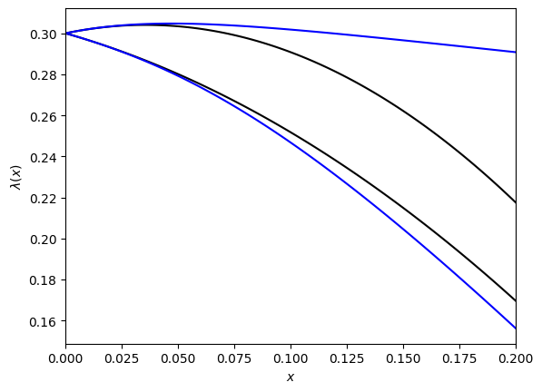
Finally plot the approximate $\lambda(x)$ (black) and compare it to the true eigenvalue (blue) (numerically computed) for real $x$:
fig, ax  = plt.subplots()
X = np.linspace(0,0.2,100)
lams =[[],[],[]]
for x in X:
    evals, evecs = np.linalg.eigh(T(x))
    for i in range(3):
        lams[i].append(evals[i])

for i in range(3):
    ax.plot(X,lam(X,i),color="black")
    ax.plot(X,lams[i],color="blue")
ax.set_xlim(0,0.2)
#ax.set_ylim(1,1.3)
ax.set_xlabel("$x$")
ax.set_ylabel(r"$\lambda(x)$")
plt.show()
Degenerate Eigenvalue Expansion
If the eigenspace to eigenvalue $\lambda$ of $T$ is not one dimensional ($\lambda$ is called a degenerate eigenvalue) and the eigenvalue $\lambda$ splits, then we look at the perturbation series (which defines an analytic function) \begin{equation} \tilde{T} (x) = \sum_{n=0}^\infty \tilde{T}_{n+1} x^n. \end{equation} The unperturbed operator here is $\tilde{T}_1$. Now $ T_r(x) = x \tilde{T} (x) $ and therefore $\tilde{\lambda}(x)$ is an eigenvalue of $\tilde{T} (x) $ if and only if $ x \tilde{\lambda}(x)$ is an eigenvalue of $T_r(x)$.
Since $\tilde{T} (x) $ is given by a perturbation series we can apply perturbation theory to it. Let $\tilde{\lambda}_{1}$ be an eigenvalue of $ \tilde{T}_{1} $ with one dimensional eigenspace. Then we can apply non degenerate perturbation theory. Assume further that $T_{1}$ is self-adjoint so $\tilde{T}_{1} = PT_{1}P$ is as well. Let $e_{1}, \dots, e_m$ be the an orthonormal basis of $\operatorname{ran}P$ which consists of eigenvectors to eigenvalue $\tilde{\lambda}_{1}, \dots, \tilde{\lambda}_m$ of $\tilde{T}_{1}$. Then this basis can be extended to a orthonormal basis $e_{1}, \dots e_m, e_{m+1}, \dots , e_n$ of $\mathcal{H}$ of eigenvectors of $T$ to eigenvalue $\lambda_{1} ,\dots, \lambda_n $, where $\lambda_{1} = \cdots = \lambda_m = \lambda$.
Let $\tilde{P}$ be the projection onto the eigenspace of $\tilde{T}_1$ to eigenvalue $\tilde{\lambda}_{1}$ then \begin{equation} \tilde{P} (-) = e_1 \langle e_1, - \rangle , \quad P(-) = \sum_{i=1}^m e_i \langle e_i , - \rangle, \quad S(-) = - \sum_{i=m+1}^n (\lambda - \lambda_i)^{-1} e_i \langle e_i, - \rangle. \end{equation} And so applying the formula from the previous section (further assuming $T_2=0$ for simplicity) \begin{equation} \operatorname{trace} \tilde{P} \tilde{T}_2 \tilde{P} = - \langle e_1 , PT_1 S T_1 P e_1 \rangle = \sum_{i=m+1}^n (\lambda - \lambda_i )^{-1} |\langle e_1, T_1e _i \rangle |^2 . \end{equation} And so there will be an eigenvalue $\lambda_1 (x)$ of $T(x)$ with \begin{equation} \lambda_1 (x) = \lambda + x \tilde{\lambda}_1 + x^2 \bigg( \sum_{i=m+1}^n (\lambda - \lambda_i )^{-1} |\langle e_1, T_1e _i \rangle |^2 \bigg) + o(x^2) . \end{equation} If all the eigenvalues of $\tilde{T}_1$ have one dimensional eigenspace, then all the eigenvalues of $T(x)$ that have split from $\lambda$ are found in this way. If not, then the degenerate expansion can be applied again to the eigenvalues in those higher dimensional eigenspaces.
Python Example
The following python jupyter notebook code illustrates the derived formula for the perturbed eigenvalues. Again a linear perturbation $T(x)= T_0 + T_1 x $ with self-adjoint $T_0$ and $T_1$ on a 3 dimensional Hilbert space is considered.
Generate the matrix (wrt to the bespoke orthonormal basis) of $T_0$ with 2-fold degenerate eigenvalue $0.3$:
deg_Eval = 0.3
l0 = [deg_Eval,deg_Eval,0.6]
T0 = np.diag(l0)
T0
array([[0.3, 0. , 0. ],
       [0. , 0.3, 0. ],
       [0. , 0. , 0.6]])
The matrix of a random perturbation $T_1$ for which $P T_1 P$ is diagonal (again in the bespoke basis):
l1 = [1-2*np.random.random(),1-2*np.random.random(),0]
T1 = np.array([[0,0,0],[0,0,0],np.random.random(size=3)])
T1 = T1+T1.T + np.diag(l1)
T1
array([[-0.31274866,  0.        ,  0.71346278],
       [ 0.        ,  0.22835368,  0.98047231],
       [ 0.71346278,  0.98047231,  0.04827524]])
Implementation of the formula for $\lambda_i (x)$ up to second order:
def lam_deg(x,i):
    l = deg_Eval + l1[i]*x
    c2  = (deg_Eval-l0[-1])**(-1)*T1[i,2]**2
    l += c2*x**2
    return l
def T(x):
    return T0+x*T1
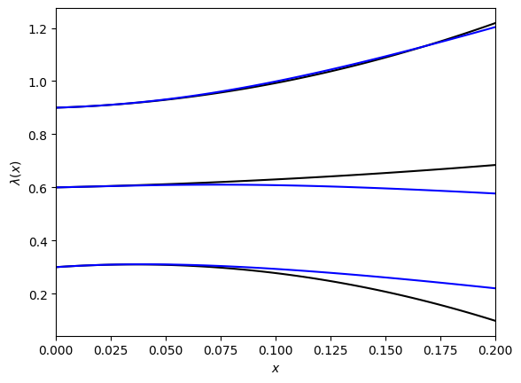
Plot the second order formula for $\lambda_i (x)$ for $i=1,2$ (black) and compare to the numeric results (blue):
fig, ax  = plt.subplots()
X = np.linspace(0,0.2,100)
lams =[[],[],[]]
for x in X:
    evals, evecs = np.linalg.eigh(T(x))
    for i in range(3):
        lams[i].append(evals[i])

for i in range(2):
    ax.plot(X,lam_deg(X,i),color="black")
    ax.plot(X,lams[i],color="blue")

ax.set_xlim(0,0.2)
ax.set_xlabel("$x$")
ax.set_ylabel(r"$\lambda(x)$")